Kruskal-Wallis is (almost) a one-way ANOVA on ranked data
Jonas Kristoffer Lindeløv
This document presents the close relationship between the Kruskal-Wallis test and one-way ANOVAs. Namely, that Kruskal-Wallis test is, to a close approximation, just a one-way ANOVA on \(rank\)ed \(y\). It is an appendix to the post “Common statistical tests as linear models”.
TL;DR: Below, I argue that this approximation is good enough when the sample size is 12 or greater and virtually perfect when the sample size is 30 or greater.
1 Simulate data
Calculate statistics for different sample sizes (\(N\)) and differences between groups (\(mu\)).
library(tidyverse)

# Parameters
Ns = c(seq(from=6, to=20, by=2), 30, 50, 80)
mus = c(0, 0.5, 1)  # Means
PERMUTATIONS = 1:200

# Run it
D = expand.grid(set=PERMUTATIONS, mu=mus, N=Ns) %>%
  mutate(
    # Generate data. One normal and one weird
    value = map2(N, mu, ~c(rnorm(.x), rnorm(.x) + .y, rnorm(.x))),
    group = map(N, ~factor(c(rep('A', .x), rep('B', .x), rep('C', .x)))),

    # Tests
    kruskal_raw = map2(value, group, ~ kruskal.test(.x ~ .y)),
    anova_raw = map2(value, group, ~aov(rank(.x) ~ .y)),

    # Tidy it up
    kruskal = map(kruskal_raw, broom::tidy),
    anova = map(anova_raw, broom::glance)
  ) %>%

  # Get as columns instead of lists; then remove "old" columns
  unnest(kruskal, anova, .sep='_') %>%
  select(-value, -group, -kruskal_raw, -anova_raw)

head(D)
2 Show results
I have found that the effect size (\(mu\)) makes no difference, so I collapse the analyses below across \(mu\).
D$N = factor(D$N)  # Make N a factor for prettier plotting

library(ggplot2)
library(patchwork)

# A straight-up comparison of the p-values
p_relative = ggplot(D, aes(x=kruskal_p.value, y=anova_p.value, color=N)) +
  geom_line() +
  geom_vline(xintercept=0.05, lty=2) +
  geom_hline(yintercept=0.05, lty=2) +

  labs(title='Absolute relation', x = 'Kruskal-Wallis p-value', y = 'ANOVA p-value') +
  #coord_cartesian(xlim=c(0, 0.10), ylim=c(0, 0.11)) +
  theme_gray(13) +
  guides(color=FALSE)

# Looking at the difference (error) between p-values
p_error_all = ggplot(D, aes(x=kruskal_p.value, y=anova_p.value-kruskal_p.value, color=N)) +
  geom_line() +
  geom_vline(xintercept=0.05, lty=2) +

  labs(title='Error', x = 'Kruskal-Wallis p-value', y = 'T-test p-value deviation') +
  theme_gray(13) +
  guides(color=FALSE)

# Same, but zoomed in around p=0.05
p_error_zoom = ggplot(D, aes(x=kruskal_p.value, y=anova_p.value-kruskal_p.value, color=N)) +
  geom_line() +
  geom_vline(xintercept=0.05, lty=2) +

  labs(title='Zoomed error', x = 'Kruskal-Wallis p-value', y = 'T-test p-value deviation') +
  coord_cartesian(xlim=c(0, 0.10), ylim=c(-0.020, 0.000)) +
  theme_gray(13)

# Show it. Patchwork is your friend!
p_relative + p_error_all + p_error_zoom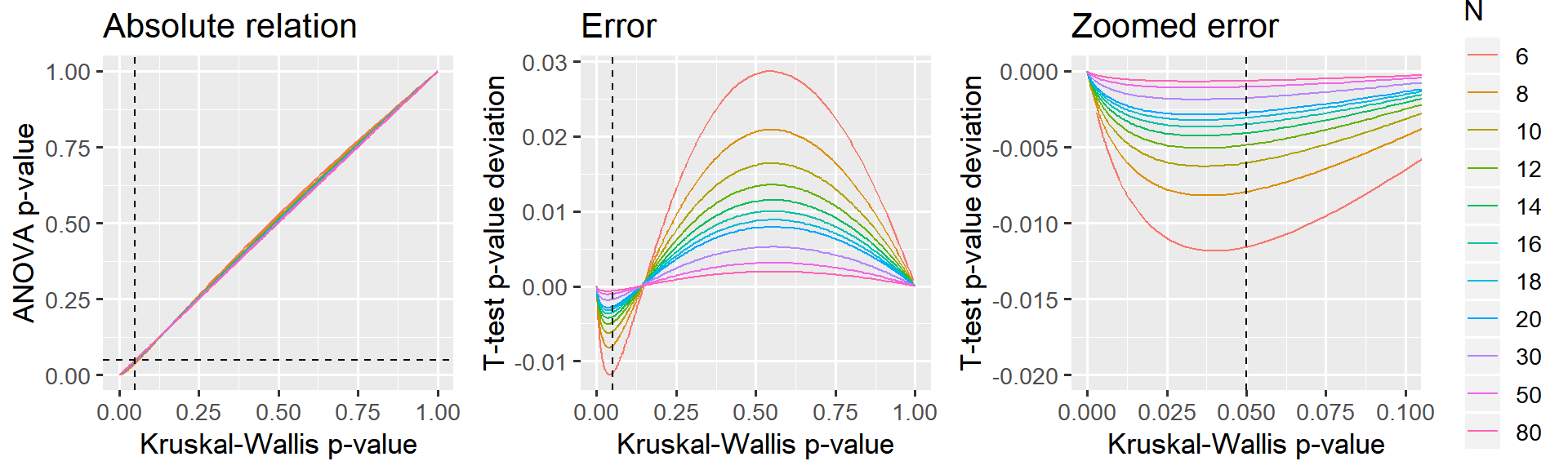
3 Conclusion
Reasonably accurate when N = 12 or greater. Almost exact when N = 30.